From Sun Glare on the Range to MCP Server: How a Golfer's First-World Problem Became an AI Tool

If you play golf, you know that the driving range is a sacred space. It is where swings are built, yardages are calibrated, and frustrations are ironed out.

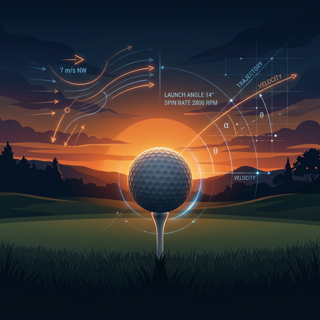
But a few days ago, I ran into a classic golfer’s first-world problem. I had a free hour in the late afternoon and wanted to hit a bucket of balls. I stepped onto the tee line at San Jose Muni range, teed up a ball, looked up, and… nothing. Just blinding, searing, low-angle afternoon sun right in my eyes. I couldn't see my ball flight, my yardages, or even where the ball landed. To make matters worse, a brutal 15 mph wind was blowing directly into my face, ballooning my shots and rendering my practice session completely useless.

As I squinted into the glare, I realized: this is a solvable data problem.

If I knew the direction the driving range was facing (its hitting azimuth), the position of the sun at this exact minute, and the current wind direction, I could calculate whether any given range was worth visiting. What started as a simple script to save myself a frustrating drive ended up becoming a full-on, production-grade Model Context Protocol (MCP) server and a dynamic web dashboard. Here is the journey of how it was built.

The Core Puzzle: Which Way Are We Hitting?

Calculating the sun’s position (azimuth and altitude) is a solved problem of orbital mechanics. Getting the wind speed and direction is a simple call to a weather telemetry API. But how do you find the hitting direction of a driving range? You can’t search Yelp for "which direction does Spartan Golf Complex face?"

To solve this, we turned to the open-source geodata engine: OpenStreetMap (OSM). By querying the OSM Overpass API, we could dynamically fetch the exact 2D boundaries (polygons) of nearby driving ranges. But a polygon is just a list of latitude and longitude coordinates. How do you convert a shape on a map into a single compass heading?

The Solution: Principal Component Analysis (PCA)
Driving ranges are naturally directional shapes—usually long, narrow rectangles or trapezoids. We can treat the coordinates of the range's boundary polygon as a 2D dataset and apply PCA.

Here is how the algorithm works under the hood:

1. Shape Coordinates: Read the OSM geometry for the driving range and get a list of (lat, lon) coordinates of the boundary of the range.
2. Bearing Calculation: Convert lat/lon points into offsets from the range centroid, then run a small PCA calculation over those points. That finds the range polygon’s longest axis, which is assumed to be the hitting corridor. Convert the result into a bearing (direction).
3. Finalize Direction: Because a long axis can point in either direction, use nearby buildings to decide which end is the tee/clubhouse side. Prefer buildings tagged as golf=clubhouse or non-residential buildings, average their coordinates into a building centroid, and compare that to the PCA vector. If the PCA vector points from the building side toward the range center, keep the bearing; otherwise flip it by 180 degrees.

Translating Math into Golf Rules

With the hitting azimuth locked in, we can apply two simple, real-world rules:

The Headwind Check: A headwind of 15 mph is only a problem if it's hitting you in the face. Calculate the effective headwind component using the cosine projection:

Where W is the wind direction angle and H is the range hitting azimuth. If the headwind component is greater than 12 mph, the range gets flagged as restricted.

The Sun Glare Check: Sun glare is only an issue when the sun is low in the sky (0 < Altitude < 20) and the difference between the sun’s azimuth and your hitting azimuth is less than 45 degrees.

From Script to Web Dashboard

Once the Python engine was working, I wanted a way to check it from my phone while on the move. I wrapped the logic in a Flask web application, building a modern dashboard available at /driving_ranges.

Using HTML5 Geolocation, the site automatically detects where you are, queries OSM for the nearest ranges, combines them with a hand-tuned local database, and spits out live, color-coded recommendations. It uses a glassmorphic dark UI with subtle glow effects, active loading skeletons, and interactive sliders to simulate different times of day.

The Final Evolution: Making it an AI Tool (MCP)

The web page was great, but the ultimate goal was to make this assistant accessible to LLMs. If I am chatting with my AI assistant about playing golf for the day, I want the AI to be able to check this for me, so the service was migrated to a Model Context Protocol (MCP) Server.

By registering the endpoint under /index.ws/mcp, any LLM client (like Cursor, Claude Desktop, or Windsurf) can connect to the server.

Now, when I ask my AI assistant: "I want to hit some golf balls around 5 PM today. Where should I go?", the AI uses the MCP server, runs the decide_golf_range tool behind the scenes, reads the PCA calculations and atmospheric vectors, and answers:

"You should head to Spartan Golf Complex. While San Jose Muni is closer, the sun will be at a 15° angle directly in your eyes at 5:00 PM, and you'll be hitting into a 14 mph headwind. Spartan faces northeast, keeping the sun at your back and the wind cross-neutral."

What started as a simple personal annoyance turned into a robust spatial recommendation engine, bridging GIS geometry, orbital math, modern web UI, and state-of-the-art AI protocol standards. Next time you head to the range, make sure the math is on your side!

Most of the heavy lifting in this project was done by AI, specifically Google Antigravity using the model Gemini 3.5 Flash (High). Minimal code editing was done in Antigravity IDE (another VS Code fork).